Calculations

We are hunting for peptides that may have taken up heavy atom isotopes such as ¹⁵N. Since there can be anywhere from 0 to maxIso uptake of heavy atoms we need to search for a range of mz's for each peptide.

We try and fit a gaussian

$$`\begin{equation} \text{norm}_{[\mu,\sigma,k,b]}(rt) = k \times e^{-( rt - \mu)^2/2 \sigma^2} + b \end{equation}`$$

to the intensities of the peptide without isotopic enrichment

$$`\begin{equation} { \color{#D63385} \text{monoFitParams} } \equiv [\hat{\mu},\hat{\sigma},\hat{k},\hat{b}] \equiv \text{minimize}_{[\mu,\sigma, k, b]} \sum_{rt} \left(k \times e^{-( rt - \mu)^2/2 \sigma^2} + b - I^{\text{mono}}_{rt} \right)^2 \end{equation}`$$

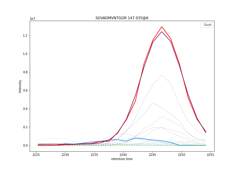
where $`I^{\text{mono}}_{rt}`$ are the intensities found for the peptide with no isotopic enrichment (see red line in diagram above). (Actually we fit to a smoothed version of the intensities)

We can use quadrature to estimate the area under this curve.

$$`\begin{equation} A^{\text{mono}} = \int_{l_b=\max(\mu_{opt} - 2 \times \sigma_{opt} , rt_0)}^{u_b=\min(\mu_{opt} + 2 \times \sigma_{opt} , rt_n)} d\text{rt} \left( k_{opt} \times e^{-(\text{rt} - \mu_{opt})^2/2 \sigma_{opt}^2}+ b_{opt} \right) \end{equation}`$$

but we use the fact that the integral of a gaussian is a scaled error function, so we can calculate this as:

$$`\begin{equation} A^{\text{mono}} = \text{b}_\text{opt} \times (u_b - l_b) + k_\text{opt} \times \sigma_\text{opt}\times \sqrt{\frac{\pi}{2}} \left[\text{erf}\left(\frac{1}{\sqrt{2}}\frac{u_b - \mu_\text{opt}}{\sigma_\text{opt}}\right) - \text{erf}\left(\frac{1}{\sqrt{2}}\frac{l_b - \mu_\text{opt}}{\sigma_\text{opt}}\right) \right] \end{equation}`$$

$`A^{\text{mono}}`$ is stored as monoPeakArea.

Also stored is a "goodness of fit" measure monoFitDiff which is the average (over retention time) of the absolute difference between the fitted curve and the observed intensities, scaled by the observed intensities (with a small epsilon to avoid division by zero).

$$`\begin{equation} { \color{#D63385} \text{monoFitDiff} } = \frac{1}{N} \frac{\sum^N_{\text{rt}\in [\text{l},\text{r}]} \vert \text{norm}_{[\hat{\mu},\hat{\sigma},\hat{k},\hat{b}]}(rt) - I_{\text{rt}}^{\text{mono}}\vert}{\left(\sum^N_{\text{rt}\in [\text{l},\text{r}]} I_{\text{rt}}^{\text{mono}}\right) + \epsilon} \end{equation}`$$

The smaller monoFitDiff is the better.

Estimating intensities of extracted ion chromatograms (EIC)s

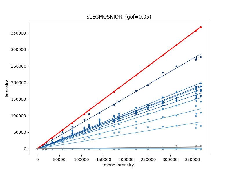
We now linearly fit the scatter plots of the heavy peptides with the base peptide. (with the configuration variable WITH_ORIGIN as False — the default — $`\alpha`$ is held to zero.)

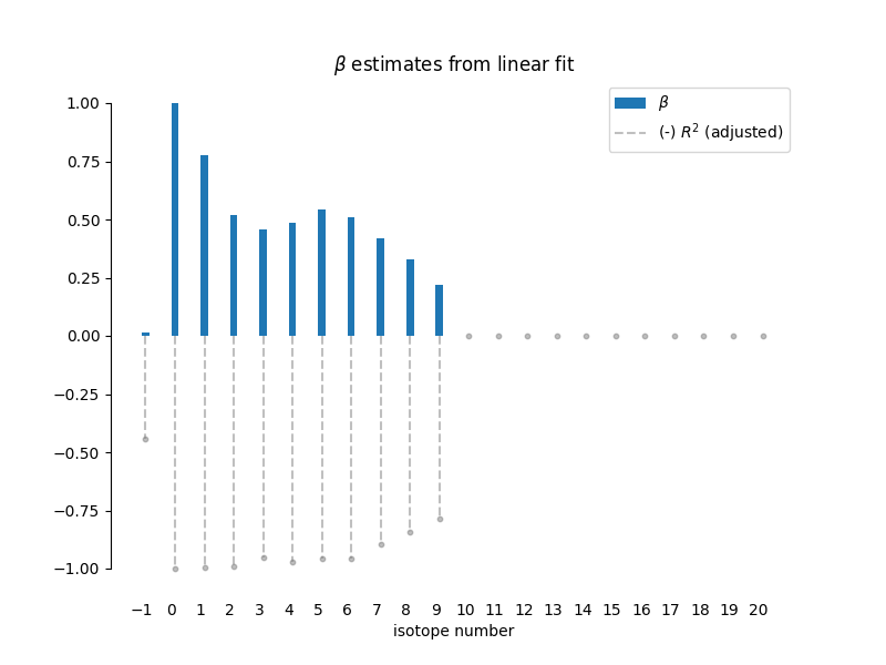
$$`\begin{equation} I^{\text{[iso]}}_{rt} \sim \alpha^{\text{[iso]}} + \beta^{\text{[iso]}} I^{\text{mono}}_{rt} \end{equation}`$$

Note that the first value of isotopeEnvelopes is based on an mz that has negative enrichment (at least theorectically!) as a check. (See the blue line in the plot at top.)

If we integrate this relationship on both sides over the retention time range we get an intensity relationship:

$$`\begin{equation} { \color{#D63385} \text{isotopeEnvelopes[iso]} } \equiv \hat{I}_{\text{iso}} = \max(0, \alpha^{\text{[iso]}} \times( u_b - l_b) + A^{\text{mono}} \times \beta^{\text{[iso]}}) \end{equation}`$$

$`\alpha`$ is probably small due to the fact that there will be zero intensities on both sides at the margins.

Also stored is goodnessOfFit that measures how well the fitted lines fits the data.

$$`\begin{equation} { \color{#D63385} \text{goodnessOfFit} } = \frac{\sum_{n > \text{mono}} (1-R^2_n) \beta^{[n]}}{\sum_{n > \text{mono}} \beta^{[n]} + \epsilon} \sim 1 -\langle R^2 \rangle \end{equation}`$$

R² is the coefficient of determination for the fitted line. The smaller the goodnessOfFit the better.

As a check we include in this calculation a "negative enrichment" point and store inv_ratio

$$`\begin{equation} { \color{#D63385} \text{inv\_ratio} } = \frac{\hat{I}_{-1}}{\hat{I}_0 + \epsilon} \sim \beta^{[-1]} \end{equation}`$$

(the smaller the better). i.e. the "negative enrichment" should be nothing.

Isotopic Abundance

The isotopic abundance of a peptide is calcualated from Efficient Calculation of Exact Fine Structure Isotope Patterns via the Multidimensional Fourier Transform (2014) by Andreas Ipsen.

There is of course a natural isotopic abundance for any peptide from all atom types (not just the one we are interested in). The calculation of this is ingenious. Since we can't measure which (say Carbon) atom in a peptide has a heavy atom, we have a combinatorial problem. With $`a_j^{[C_n]}`$ as the abundance fraction of isotope j on (Carbon) atom n we calculate the abundance profile for all (Carbon) atoms on the peptide as (we assume zeros outside the isotopic abundance range):

$$`\begin{equation} \begin{split} \text{a}^{[C]}_i =& \sum_{i=j+k+l+\cdots+z} a^{[\text{C}_1]}_{j} a^{[\text{C}_2]}_k a^{[\text{C}_3]}_l \times \cdots \times a^{[\text{C}_N]}_z \\ \equiv& \sum_{k,l,\cdots,z} a^{[\text{C}_1]}_{i-k+l+\cdots+z} a^{[\text{C}_2]}_k a^{[\text{C}_3]}_l \times \cdots \times a^{[\text{C}_N]}_z \end{split} \end{equation}`$$

(The abundances of each isotope of an element must sum to 1).

But this is a discrete convolution which, when (discrete) fourier transformed, becomes a "simple" product.

$$`\begin{equation} \implies \mathcal{FFT}\{\text{a}^{[C]}\}_k = \left[\sum_j a_j^{[C]} e^{-\frac{2\pi i j k}{M}}\right]^N \end{equation}`$$

So the full abundance profile (which we call ndist) is the inverse FFT of this:

$$`\begin{equation} { \color{#D63385} \text{ndist}}_{[a^{[C]},a^{[N]},...]} \approx \sum_{i=k+l+m+n+\dots} a^{[\text{C}]}_k a^{[\text{N}]}_l a^{[\text{S}]}_m a^{[\text{P}]}_n\dots \end{equation}`$$

Since this too is a convolution we can calculate it by the pointwise product of the FFTs (see above) before doing the final inverse FFT.

We use this a lot since we need to calculate it with elevated abundance levels for the isotope we are using in our experiment. We use the notation $`{ \color{#D63385} \text{ndist}}_{[E]}`$ to identify the abundances found if the environmental abundance (of our heavy isotope is E).

We calculate isotopic abundance from natural abundance to (user specified) maximum labelled abundance

$$`\begin{equation} a_i = \text{natural-abundance}^\text{0} + \frac{i}{N -1}\times(\text{maximumLabelEnrichment} - \text{natural-abundance}^\text{0}) \quad\forall\; i \in [0,N-1] \end{equation}`$$

where N is usually 10 but can be specified in the TurnoverJob file in [settings] as enrichmentColumns. Then we adjust abundances of the labelled element (so they always sum to 1)

$$`\begin{equation} \text{adjustedAbundance}_{k}^\text{iso} = \left\{ \begin{array}{ll} (1-a) \times \frac{\text{natural-abundance}^k}{\sum_{l\ne \text{iso}} \text{natural-abundance}^l} & \text{if}\; \text{iso} \ne k \\ a\; & \text{if}\; \text{iso} = k\end{array}\right. \quad k \in \text{isotopes of labelled element} \end{equation}`$$

(iso identifies the isotope number of the labelled element, e.g. ¹⁵N)

for each of these values we recalulate the ndist array with these new abundances.

$$`\begin{equation} \begin{array}{cc} & \begin{array}{ccc} \quad a_o & a_1 & \cdots & a_{N-1} \\ \end{array} \\ \begin{array}{r c c} \text{iso}_0 \\ \text{iso}_1 \\ \text{iso}_2 \\ \cdots \\ \text{iso}_{\text{isoMax}} \end{array} & \left[ \begin{array}{c c c} \left[\begin{array}{c} \color{red}{n} \\ \color{red}{d} \\ \color{red}{i} \\ \color{red}{s} \\ \color{red}{t} \end{array} \right] \left[\begin{array}{c} \color{green}{n} \\ \color{green}{d} \\ \color{green}{i} \\ \color{green}{s} \\ \color{green}{t} \end{array} \right] \;\cdots\; \left[\begin{array}{c} \color{blue}{n} \\ \color{blue}{d} \\ \color{blue}{i} \\ \color{blue}{s} \\ \color{blue}{t} \end{array} \right] \end{array} \right] \end{array} \begin{array}{c} \; \\ \times \mathbf{w} \end{array} \begin{array}{c} \; \\ \quad = \end{array} \begin{array}{c} \; \\ \quad \mathbf{M} \times \mathbf{w} \end{array} \begin{array}{c} \; \\ \quad \sim \end{array} \begin{array}{c} \; \\ \quad \mathbf{\hat{I}}_{\text{iso}} \end{array} \end{equation}`$$

where the matrix $`\bf{M}`$ can be visualised as:

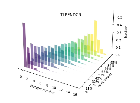
with "isotope number" the matrix rows and "enrichment" the columns (note how the isotope number goes up as the enrichment increases).

With $`\mathbf{w} \ge 0`$ and $`\text{labelledEnvelopes} \equiv \mathbf{w}`$. We do a Non-Negative Least Squares (NNLS) optimisation to estimate the $`\mathbf{\hat{w}}`$.

We calcuate a scaled deviance as a measure of goodness of fit. (Stored as nnls_residual -- the numerator -- and totalNNLSWeight -- the denominator -- in the database)

$$`\begin{equation} \frac{\sqrt{\Vert \mathbf{M} \times \mathbf{\hat{w}} - \mathbf{\hat{I}}_{\text{iso}} \Vert^2}}{\sum_i \hat{w}_i } \end{equation}`$$

If we turn the positive weights $`\mathbf{\hat{w}}`$ into fractions $`f_i = w_i / \sum_{i=0}^{N-1} w_i`$ then LPF $`\equiv \text{relativeIsotopeAbundance}`$ (an estimate of the fraction of this peptide that include some/any heavy atoms)

$$`\begin{equation} \text{relativeIsotopeAbundance} = \sum_{i \ge N \times \text{lpfPercent}}^{N-1} f_i \end{equation}`$$

where lpfPercent is a configuration variable (in [settings] default: 0.1) and N is enrichmentColumns (default: 10).

This — with default values — is usually just:

$$`\begin{equation} \text{relativeIsotopeAbundance} = 1 - f_0 \end{equation}`$$

enrichment is an estimate/average of the fraction of heavy atoms (of the labelled type) in the peptide:

$$`\begin{equation} \text{enrichment} = \langle a_i \rangle = \sum_{i=0}^{N-1} f_i a_i \ge 0 \end{equation}`$$

where $`N`$ is usually 10 but can be specified in the TurnoverJob file in [settings] as enrichmentColumns.

We also store two correlations

and

where $`\rho`$ is pearson correlation coefficient.

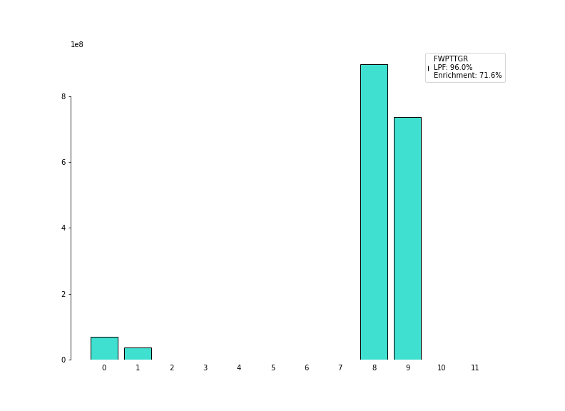
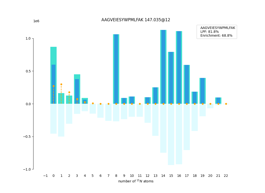
Fitted Envelopes Plot

With E as enrichment and relativeIsotopeAbundance as LPF we calculate :

$$`\begin{equation} \text{theoreticalDist} = \mathbf{M} \times \mathbf{\hat{w}} \end{equation}`$$

• naturalDist = $`I_0 \times`$ natural distribution of "extra" neutrons is plotted as orange vertical dashed lines.
• theoreticalDist is mirrored on the x-axis and plotted inverted as .
• isotopeEnvelopes is plotted as
• the negative enrichment value is used to filter hits $`\frac{\text{isotopeEnvelopes}[0]}{\text{isotopeEnvelopes}[1]} \lt \text{monoMinus1MaxRatio}`$

Data Cull

Once all the computations are done we need to select "good" data .

This is controlled by the background protein-turnover configuration value:

GOOD_PEPTIDES = """
      (inv_ratio < {maxCullScore}/5.0)
    & (nnls_residual/totalNNLSWeight < {maxCullScore})
    & (goodnessOfFit < {maxCullScore})
    & (monoFitDiff < {maxCullScore})
"""

Since we don't really care about the peptides charge state, modifications etc. we then group on the "peptide" column and select the row with the maximum "maxPeakArea". This is controlled by the background configuration value:

DEDUP_WITH = ["peptide", "maxPeakArea"]

All values are evaluated using pandas eval so you could change this with (viz: dedup.toml)

DEDUP_WITH = ["peptide", "maxPeakArea/monoPeakArea"]

And then run turnover --config=dedup.toml run somejob.toml.

This would ensure that you selected the largest maxPeakArea/monoPeakArea value for each group of peptides.